

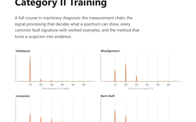
Vibration Analysis Training: Category II
An 88-page course book on vibration diagnosis: which fault produces which pattern, what phase adds, and how to disprove an answer before reporting it.
Enter Fmax, the line count, the window and the averaging scheme, and the calculator gives you the bin spacing, the separation two peaks really need, the time each block takes and the total time on the machine. Lines of resolution get quoted everywhere. The separation the setup will actually deliver gets quoted almost nowhere, and for the window nearly everyone uses it is half as much again as the bin spacing.
With Fmax in hertz and lines the number of spectral lines:
With a shaft speed in rpm, two more follow, where fr = rpm / 60:
A window function tapers each block of data to zero at both ends so that the block can be treated as one period of a repeating signal. The price is that a single frequency component no longer lands in one bin. It spreads, and the noise equivalent bandwidth says how far.
| Window | Where it belongs | What it costs |
|---|---|---|
| Hanning | General analysis of a running machine | Amplitude error up to about 16 percent on a peak between bins |
| Flat top | Calibration and amplitude-critical readings | Much poorer frequency resolution |
| Rectangular (none) | A transient contained wholly inside the block | Severe leakage on any continuous signal |
| Exponential | A bump test ring-down | Adds artificial damping to the result |
The separation figures the calculator uses, about 1.5 bins for Hanning, close to 4 for flat top and 1 for no window at all, are the published noise equivalent bandwidths of those window shapes. They are working numbers, not values a standard fixes.
Flat top is the trade that catches people out. It measures amplitude accurately, which is exactly what you want when calibrating or balancing, and it costs you nearly four bins of separation to do it. Run a flat top window on a routine route and closely spaced peaks that a Hanning window would have separated will merge into one.
The exponential window has no separation figure at all, which is why the calculator withholds one when it is selected. What it costs is damping rather than bins, and the amount depends on the decay constant and on frequency, so it is calculated for the measurement rather than looked up. Correct for it before quoting a damping ratio: at low frequency the window can contribute more damping than the mode has.
Block time is the reciprocal of bin spacing, and nothing negotiates that away. Halving the bin spacing doubles the seconds the analyst stands at the machine, for every average.
Overlap is what makes averaging affordable. At 50 percent, each average after the first advances the record by half a block; at 75 percent, by a quarter. Four averages with no overlap take four block times; the same four at 50 percent take 2.5. Eight at 75 percent take 2.75 rather than eight, which is a little over a third of the time and not a quarter of it: the first block is paid for in full whatever the overlap, and it is the seven after it that are cheap. What you give up is independence: overlapped averages share samples, so they do not reduce random noise as effectively as the same number of fresh blocks would.
Analysers sample at 2.56 times Fmax rather than the theoretical minimum of twice, because the anti-alias filter needs a band above Fmax to roll off in. The same factor converts lines into samples, which is why familiar line counts produce familiar powers of two: 400 lines is 1024 samples, 1600 lines is 4096.
Most arguments about line counts are really one question: will sidebands at shaft speed resolve?
Sidebands around a bearing or gear frequency are spaced at shaft speed, and they carry the diagnosis. Compare the shaft frequency with the real separation. Three times the separation or more is comfortable. Between one and a half and three times, the sidebands show as shoulders on the main peak rather than as separate peaks. Below one and a half times, they do not resolve at all, and the fix is to raise the line count or lower Fmax rather than to look harder.
On a slow machine this is what forces the line count up, and it is worth noticing that lowering Fmax achieves the same thing at no cost in time, provided nothing above the new Fmax matters.
Fmax 1000 Hz, 1600 lines, Hanning window, 4 averages at 50 percent overlap, on a shaft turning at 1480 rpm.
Sidebands at shaft speed sit 24.67 / 0.9375 = 26.3 times the real separation apart. They will resolve with room to spare.
Now put the same setup on a shaft turning at 100 rpm. The shaft frequency is 1.67 Hz, and 1.67 / 0.9375 is 1.8, which is marginal: the sidebands will appear as shoulders. Doubling to 3200 lines halves the bin spacing to 0.3125 Hz and the separation to 0.46875 Hz, which puts the ratio at 3.6 and resolves them properly. It also doubles the block time to 3.2 seconds, which is the whole of the argument in one line: on slow machines, resolution is paid for in minutes.
Bin spacing is Fmax divided by the number of lines of resolution. A 1000 Hz spectrum taken with 1600 lines has bins 0.625 Hz apart. That is not the same as the separation two peaks need in order to appear as two peaks, because the window function spreads every peak across more than one bin. With a Hanning window the usable separation is 1.5 times the bin spacing, so 0.9375 Hz in that example.
Lines of resolution set how finely the spectrum is divided; the window function sets how finely it can actually distinguish. Every window spreads a single frequency component across a group of bins, and its noise equivalent bandwidth says how many. The published figures for the common shapes are about 1.5 bins for Hanning and close to 4 for flat top, against 1 for no window at all. Multiply the bin spacing by that figure to get the separation two components genuinely need. Those are properties of the window shapes rather than anything a standard fixes, so treat them as the working numbers they are.
The sampling theorem sets a floor of twice the highest frequency of interest, but a real anti-alias filter cannot cut off vertically at that frequency. Sampling at 2.56 times Fmax leaves a band above Fmax for the filter to roll off in, so energy that would otherwise fold back into the spectrum is attenuated before it is digitised. The same factor turns a line count into a block length: 1600 lines is 4096 samples.
Hanning for routine spectra on a running machine, because it separates closely spaced components better than the alternatives that get the amplitude right, at a cost of up to about 16 percent in amplitude on a peak that falls between bins. Flat top when the amplitude itself has to be accurate, such as during calibration or a balancing run, accepting that it needs far more separation between peaks. Rectangular, meaning no window at all, only for a transient contained wholly inside the block. Exponential for a bump test ring-down.
Not rectangular, which is the common mistake. The ring-down does not finish inside the block, so with no window the record is cut off mid-decay and leaks badly, and with a Hanning window part of the ring-down is thrown away. The answer is an exponential window on the response channel, which forces the decay to zero before the block ends, and a rectangular window on the force channel if an instrumented hammer is being used. Without a force channel, capture the response alone and read the peaks. The exponential window adds damping of its own, by a calculable amount, and that has to be removed before any damping figure is quoted.
Yes, and it costs something. With no overlap each average needs its own fresh block of data, so eight averages take eight block times. At 50 percent overlap each average after the first advances the record by half a block, and at 75 percent by a quarter, so eight averages take 4.5 and 2.75 block times respectively. The saving is real, but overlapped averages share samples and are no longer statistically independent.
The calculator gives you the number. These course books explain what the number means and how the measurement that produced it should be taken.
An 88-page course book on vibration diagnosis: which fault produces which pattern, what phase adds, and how to disprove an answer before reporting it.
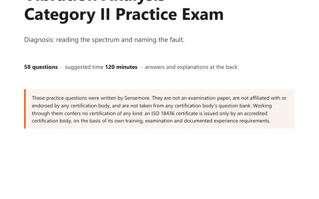
58 practice questions on vibration diagnosis, from fault signatures and phase to bearings, gears and resonance, each answer worked rather than lettered.
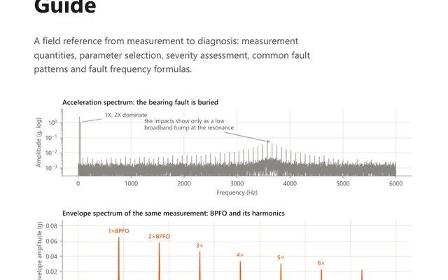
A 15-page field reference for the analyst on the route: measurement parameters, severity assessment, annotated fault spectra and bearing frequency formulas.